Our AI Syllabus project at Purdue SPARK Lab is now at the fine-tuning stage. As I am learning the basics of fine-tuning, I want to share what I have learned so far in this article.
Fine-tuning is the process of taking a pre-trained model and training it further on a specific dataset so it performs better on a particular task. The overall process looks like this:
Data Preparation → Training Configurations → Training Loop → Evaluation
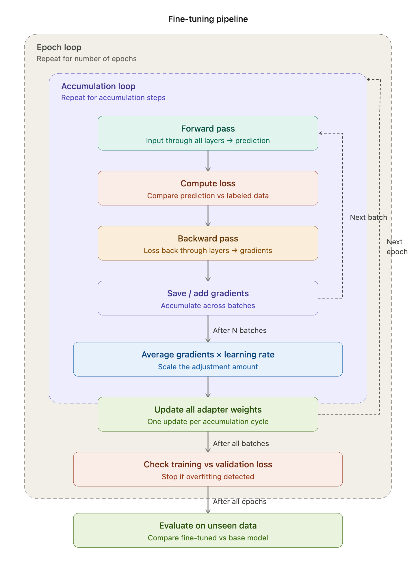 Fig. 1: The overall fine-tuning process (Claude Diagram)
#Key Terms
Before we dive in, here are some key terms that will come up throughout the article:
- Parameters / Weights: The numbers inside the model that get adjusted during training. A model’s size (e.g. 7B parameters) refers to how many of these it has.
- Layer: A building block of the model. Each layer receives input, transforms it using its weights, and passes the result to the next layer. For example, Llama 2 7B has 7 billion parameters spread across 32 transformer layers.
- Loss: A single number measuring how wrong the model’s prediction is.
- Gradient: The signal that tells the training process which direction to adjust parameters to reduce loss.
- Hyperparameters: Knobs set manually before training (e.g. learning rate, batch size).
- Backpropagation (Backward pass): Algorithm that calculates the gradient for every weight in the model.
- Tokenization: Converting text into a sequence of numeric IDs (tokens) that the model can process.
- Overfitting: Model memorizes training data instead of learning general patterns.
- Regularization: Techniques that fight overfitting.
Now let’s walk through each step of the fine-tuning process.
#Data Preparation
Data quality over quantity. In practice, we only need a surprisingly small amount of data to fine-tune the model, as it already knows grammar, logic, and other fundamentals. Therefore, the quality is the most important factor as it can directly impact our model results.
A good quality dataset means every example should follow the exact same format and the outputs should be what we want from the model. For example, the popular Alpaca dataset uses this structure:
{
  "instruction": "Summarize the following paragraph.",
  "input": "The Federal Reserve raised interest rates by 25 basis points...",
  "output": "The Fed raised rates by 0.25%, signaling continued efforts to control inflation."
}
Every single example follows the same instruction/input/output format, and the outputs match the style we want the model to produce.
#Training Configurations
Once the data is ready, we set the hyperparameters — the knobs that control how the model learns. Here are some of the hyperparameters:
| Hyperparameter | What it does | Typical value | Too high | Too low |
|---|---|---|---|---|
| Learning rate | Size of each weight adjustment step | 2e-5 | Unstable training, catastrophic forgetting | Barely learns anything, wastes compute |
| Epochs | Number of full passes through the dataset | 2–3 | Overfitting (memorizes data) | Underfitting (hasn’t learned enough) |
| Batch size | Number of samples processed before one weight update | 2–4 (with gradient accumulation) | Out of memory | Noisy, unstable gradient estimates |
| Gradient accumulation steps | Simulates larger batch by summing gradients over multiple steps | 4–8 | Slower training, diminishing returns | Same problems as small batch size |
| Warmup steps | Gradually ramps learning rate up from ~0 at the start | 5–10% of total steps | Wastes training time learning slowly | Early instability, loss spikes at start |
| Weight decay | Penalizes large weights to prevent overfitting | 0.01 | Underfitting (over-regularized) | More prone to overfitting |
Among these, two are worth explaining further:
- Epochs: If you have 1,000 training examples and set epochs to 3, the model will go through all 1,000 examples three times — that is 3 full passes through the entire dataset.
- Batch size: Instead of updating weights after every single example, the model processes a small group (batch) at a time. A batch size of 4 means the model looks at 4 examples, averages what it learned, and then makes one weight update.
#How Gradients Are Computed
Now that we know what batch size is, let’s see how it connects to the other hyperparameters during a weight update.
The process works in three steps:
- The model computes gradients for each batch — these tell us which direction to adjust the weights.
- If gradient accumulation is enabled, the model repeats this over multiple batches and averages the gradients together. This simulates a larger batch without needing more memory. For example, with a batch size of 2 and 8 accumulation steps, the model processes 2 × 8 = 16 examples before making one weight update.
- The averaged gradient is then multiplied by the learning rate to determine the actual size of the adjustment. If the gradient says “move the weight down by 0.5” and the learning rate is 2e-5, the actual adjustment is 0.5 × 0.00002 = 0.00001 — a very small, controlled step.
#Training Loop
With the data prepared and hyperparameters set, the training loop is where the model actually learns.
Fine-tuning is basically correcting the model’s prediction over and over again by adjusting the weights. The model compares its prediction with the actual labeled data to calculate the loss (how wrong), computes the gradient (which way to fix), and adjusts the weights.
Each training step follows this cycle:
Predict (Forward) → Loss → Gradient (Backward) → Adjust Weights → Repeat
Every step has a forward pass and a backward pass in pairs:
- Forward pass — input flows through all the layers in order → produces a prediction → computes the loss
- Backward pass — the loss flows back through all the layers in reverse order → computes gradients for every weight
Putting it all together with epochs and gradient accumulation from earlier:
Epoch loop (repeat N times over the full dataset)
    Accumulation loop
        Batch
            Forward pass → Loss → Backward pass (compute gradients)
Average accumulated gradients → multiply by learning rate → update weights#Frameworks
In practice, we do not write the training loop from scratch. These libraries handle it:
- Transformers (HuggingFace) — loads the model and tokenizer.
- PEFT — adds parameter-efficient adapters onto the model (only for LoRA method).
- TRL — provides the SFTTrainer that runs the actual training loop.
#Evaluation
After training completes, we need to check whether the model actually learned or just memorized.
We check for overfitting by splitting the data into training and validation sets and comparing training loss vs. validation loss. If training loss goes down but validation loss goes up, that means the model is only memorizing the data, not actually learning generalizable patterns.
That covers the fundamentals of fine-tuning — from data preparation to training and evaluation. For our AI Syllabus project, we are using LoRA (Low-Rank Adaptation), a parameter-efficient method that freezes the original model weights and only trains small adapter matrices on top. In the next article, I will dive deeper into how LoRA works and walk through the actual code.