As we have learned the technical nuts and bolts of fine-tuning in Fine-Tuning (1): Basics and Fine-Tuning (2): LoRA, have you ever wondered what the fine-tuning process actually looks like in real life? Can we even do it on our own at home? With all that curiosity, I ran my first fine-tuning experiment using the TinyLlama-1.1B-Chat model and the public Alpaca dataset.
In this article, I will unwrap the magical fine-tuning box and walk through the code. The full notebook is available on my GitHub.
As we discussed previously, fine-tuning follows this process: Setup → Load Model → Load Dataset → Configuration (LoRA and Training) → Training → Test
#Setup
The entire notebook runs on a free Google Colab T4 GPU — no local setup needed.
First, confirm the GPU is available:
!nvidia-smiInstall the libraries we covered in the previous articles (transformers for the model, peft for LoRA, trl for the training loop):
!pip install transformers peft trl datasets accelerate bitsandbytes -q#1. Load the Model and Tokenizer
We are using TinyLlama-1.1B-Chat — a 1.1B parameter model that fits comfortably on a free Colab GPU. Its small size makes it ideal for a first run where the goal is to learn the pipeline, not squeeze out performance.
from transformers import AutoModelForCausalLM, AutoTokenizer

model_name = "TinyLlama/TinyLlama-1.1B-Chat-v1.0"
tokenizer = AutoTokenizer.from_pretrained(model_name)
model = AutoModelForCausalLM.from_pretrained(
    model_name,
    torch_dtype=torch.float16,
    device_map="auto"
)
A few things worth pointing out:
AutoModelForCausalLMandAutoTokenizercome from HuggingFace’stransformerslibrary. They always get loaded in pairs — the tokenizer has to match the model it was trained with.torch_dtype=torch.float16loads the weights in half precision, cutting memory usage in half (covered in the Quantization section of Fine-Tuning (2): LoRA).device_map="auto"lets HuggingFace place the model on the GPU automatically.
#2. Load and Split the Dataset
We are using tatsu-lab/alpaca — the same instruction-following dataset from Fine-Tuning (1): Basics, where every example follows a clean instruction/input/output format.
Here is what a single example looks like:
Below is an instruction that describes a task. Write a response that appropriately completes the request.

### Instruction:
Give three tips for staying healthy.

### Response:
1. Eat a balanced diet and make sure to include plenty of fruits and vegetables.
2. Exercise regularly to keep your body active and strong.
3. Get enough sleep and maintain a consistent sleep schedule.
Note that this dataset only contains instruction and output (the response) — there is no separate input field. The first sentence is the system prompt that frames the task for the model.
from datasets import load_dataset

dataset = load_dataset("tatsu-lab/alpaca", split="train")
print(len(dataset))
print(dataset[0])
The full dataset has ~52k examples, which is way more than we need for a first run. We shuffle with a fixed seed (for reproducibility), grab 1,000 examples, and do an 80/20 train/validation split:
dataset = dataset.shuffle(seed=42).select(range(1000))

split = dataset.train_test_split(test_size=0.2, seed=42)
train_dataset = split["train"]
val_dataset = split["test"]

print(f"Training examples: {len(train_dataset)}")
print(f"Validation examples: {len(val_dataset)}")
That leaves us with 800 training examples and 200 validation examples. The validation set is what we use to check for overfitting — if training loss keeps dropping but validation loss starts rising, that’s our signal the model is memorizing instead of learning.
#3. Configure LoRA
This is where the peft library comes in. In Fine-Tuning (2): LoRA, we walked through the math behind LoRA — how two small matrices A and B approximate the weight update ΔW = B × A. This is where we actually plug it into the model.
from peft import LoraConfig, get_peft_model

lora_config = LoraConfig(
    r=16,
    lora_alpha=32,
    target_modules=["q_proj", "k_proj", "v_proj", "o_proj"],
    lora_dropout=0.05,
    bias="none",
    task_type="CAUSAL_LM"
)

model = get_peft_model(model, lora_config)
model.print_trainable_parameters()
Breaking down the config:
r=16— the rank of the LoRA adapters. A standard starting value.lora_alpha=32— scaling factor, set to 2 × r as recommended in “Fine-Tuning (2): LoRA”.target_modules— attach adapters to the four attention projection layers: query, key, value, and output. These are the layers LoRA typically targets.lora_dropout=0.05— light regularization to prevent the adapters from overfitting.bias="none"— don’t train the bias terms, only the A and B matrices.task_type="CAUSAL_LM"— tells PEFT this is a causal (next-token-prediction) language model.
After get_peft_model, the base TinyLlama weights are frozen and only the LoRA adapter weights are trainable. print_trainable_parameters() reports exactly how many parameters we are actually training versus the total.
The first time I ran this cell, I was shocked — only roughly 0.4% of the parameters were trainable, while the remaining 99.6% stayed frozen. That is exactly why LoRA is so memory-efficient.
#4. Training Configuration
With the model wrapped and ready, we configure the training run using trl’s SFTConfig:
from trl import SFTConfig, SFTTrainer

training_config = SFTConfig(
    output_dir="./results",
    num_train_epochs=3,
    per_device_train_batch_size=4,
    gradient_accumulation_steps=4,
    learning_rate=2e-4,
    warmup_steps=10,
    weight_decay=0.01,
    logging_steps=10,
    eval_strategy="steps",
    eval_steps=50,
    save_strategy="steps",
    save_steps=50,
    fp16=True,
    dataset_text_field="text",
)
Most of these should look familiar from Fine-Tuning (1): Basics. A few things worth noting for this specific run:
num_train_epochs=3— three full passes over the 800 training examples.per_device_train_batch_size=4withgradient_accumulation_steps=4— effective batch size of 16, exactly the pattern we covered in “Fine-Tuning (1): Basics”.learning_rate=2e-4— this is higher than the 2e-5 typical for full fine-tuning. LoRA adapters are small and randomly initialized, so they tolerate (and benefit from) larger steps.fp16=True— train in half precision to save memory.eval_steps=50— run validation every 50 steps so we can watch training loss and validation loss side by side in real time.save_steps=50— save a checkpoint every 50 steps, so we can recover if training crashes or pick an earlier checkpoint if later ones overfit.
#5. Run the Training
Everything comes together in the SFTTrainer:
trainer = SFTTrainer(
    model=model,
    args=training_config,
    train_dataset=train_dataset,
    eval_dataset=val_dataset,
    processing_class=tokenizer
)

trainer.train()
We pass in the LoRA-wrapped model, the training config, both datasets, and the tokenizer. Then .train() runs the full loop — forward pass → loss → backward pass → weight update → repeat — exactly as described in Fine-Tuning (1): Basics.
During training, logs print every 10 steps showing training loss, and an evaluation runs every 50 steps showing validation loss.
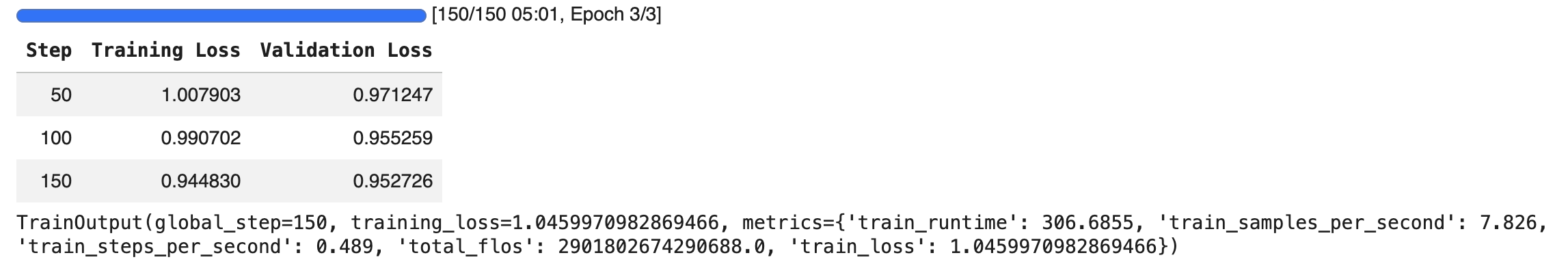 Fig. 1: TinyLlama + Alpaca training run — total batches, epochs, and runtime on top, with training and validation loss plotted every 50 steps
The screenshot above shows what I got after training finished. The top bar reports the total number of batches, epochs, and runtime. The chart plots training loss and validation loss every 50 steps, and we can see a smooth decrease in both. The gap between training and validation loss stays small, which is a good sign that the model is not overfitting.
#6. Test It Out
Once training finishes, the fine-tuned model is ready to use. Here is a simple helper for generation:
def generate_response(prompt, model, tokenizer):
    inputs = tokenizer(prompt, return_tensors="pt").to(model.device)
    outputs = model.generate(
        **inputs,
        max_new_tokens=200,
        temperature=0.7,
        do_sample=True,
    )
    response = tokenizer.decode(outputs[0], skip_special_tokens=True)
    return response
One important detail: we format prompts using the same Alpaca instruction template the model was trained on. Matching the training format matters — if we prompt it in a different structure, the model has no reason to behave like a fine-tuned instruction follower.
prompt = """Below is an instruction that describes a task. Write a response that appropriately completes the request.

### Instruction:
Explain what fine-tuning a language model means in simple terms.

### Response:
"""
print(generate_response(prompt, model, tokenizer))
The returned output is:
### Response:
Fine-tuning a language model involves repeatedly training a model on additional data, typically augmented with new examples to improve its ability to understand and generate natural language. This process is known as "fine-tuning" and it is an essential step in the process of building a machine learning model for natural language processing.
You can repeat this with any other Alpaca-style prompt — the notebook has a second example asking about the benefits of regular exercise.
#Reflections
That wraps up the full LoRA fine-tuning walkthrough. The entire process is straightforward and easy to follow once you understand the underlying concepts. On top of that, most of the code is boilerplate — the libraries do almost all the heavy lifting:
Transformers → model. PEFT → LoRA. TRL → training loop.
#Next Steps
Even though the code is rather straightforward, fine-tuning quality depends heavily on the dataset. A good dataset is what actually makes or breaks the result.
Since the Alpaca dataset came pre-formatted, the training was fairly easy. In the next article, I will share the process of taking a real-world dataset and converting it into a trainable format, along with using QLoRA and the Unsloth library to save more memory during experimentation.