In Fine-Tuning (1): Basics, I mentioned that we are using LoRA (Low-Rank Adaptation) to train our model. In this article, I will explain how LoRA works, how quantization reduces memory usage, and how QLoRA combines both. In the next article, I will walk through the actual training code.
#Key Terms
Before we dive in, here are some key terms that will come up throughout the article:
- Parameters / Weights: The numbers inside the model that get adjusted during training. A model’s size (e.g. 7B parameters) refers to how many of these it has.
- Layer: A building block of the model. Each layer receives input, transforms it using its weights, and passes the result to the next layer.
- Overfitting: When a model memorizes training data instead of learning general patterns.
- Adapters: Small trainable matrices attached to the fixed original weights. Only these get updated during LoRA fine-tuning.
- Rank: In linear algebra, the rank of a matrix measures how much independent information it contains. A low-rank matrix can be decomposed into smaller matrices with minimal information loss.
- PEFT (Parameter-Efficient Fine-Tuning): A family of methods (including LoRA) that fine-tune only a small subset of parameters instead of the entire model.
#Full Fine-Tuning vs. LoRA
Full fine-tuning updates all of the model’s original weights directly. While more powerful, it requires massive GPU memory since gradients must be stored for every single parameter.
LoRA (Low-Rank Adaptation) takes a different approach: it freezes all original weights and attaches small new adapter matrices to specific layers. Only these tiny adapters get trained, so the original model stays completely untouched.
Here is how they compare:
| Full Fine-Tuning | LoRA | |
|---|---|---|
| What changes | All original weights | Only small adapter matrices (original weights frozen) |
| Memory | ~56GB+ VRAM for a 7B model | ~16GB for the same 7B model |
| Speed | Slower — computes gradients for all parameters | Faster — only computes gradients for the small adapters |
| Output | A whole new model | A tiny adapter file (~10–100MB) on top of the base model |
| Libraries | Transformers + TRL | Transformers + TRL + PEFT |
In short, LoRA leaves the original model untouched while being faster and using less memory than full fine-tuning.
#Quantization
Before we get into how LoRA works, we need to understand quantization — it is key to how QLoRA saves so much memory.
Quantization is about representing numbers with fewer bits. Every weight in a model is just a number like 0.0023847. The question is: how many bits do we use to store it?
| Precision | Bits per weight | Memory for a 4B model |
|---|---|---|
| Full precision (float32) | 32 bits (4 bytes) | 16 GB |
| Half precision (float16) | 16 bits (2 bytes) | 8 GB |
| 4-bit quantization (NF4) | 4 bits (0.5 bytes) | ~2 GB |
Most models today use half precision (float16) by default. 4-bit quantization goes further — it maps every weight to one of only 16 possible values, saving 75% of memory compared to float16.
The tradeoff is precision: with fewer bits, the stored values are approximations of the originals. But research has shown that this small loss in precision barely affects model performance, while the memory savings are massive. This tradeoff is what makes QLoRA possible — we will see how in the next section.
#How LoRA Works
In the previous article, we learned that fine-tuning adjusts weights through a cycle of forward pass → loss → backward pass → weight update. Full fine-tuning updates the entire weight matrix W directly. LoRA’s key insight is: what if we don’t need to update the full matrix?
Instead of modifying W (which could be massive), LoRA freezes it and injects two small trainable matrices, A and B, alongside it. The weight update is approximated as ΔW = B × A, where A has shape r × k and B has shape d × r. The rank r is tiny (typically 8, 16, or 32), so the number of trainable parameters drops dramatically.
For example, consider a 512 × 512 weight matrix — that’s 262,144 parameters to update with full fine-tuning. With LoRA at rank 8, we instead train A (8 × 512) and B (512 × 8), which is only 8,192 parameters — a 97% reduction. The product B × A still produces a 512 × 512 matrix, so it can be added directly to the original W.
![]() Fig. 1: LoRA low-rank decomposition — instead of updating the full 512 × 512 matrix, we train two smaller matrices A and B
Fig. 1: LoRA low-rank decomposition — instead of updating the full 512 × 512 matrix, we train two smaller matrices A and B
Here is what the training loop looks like with LoRA:
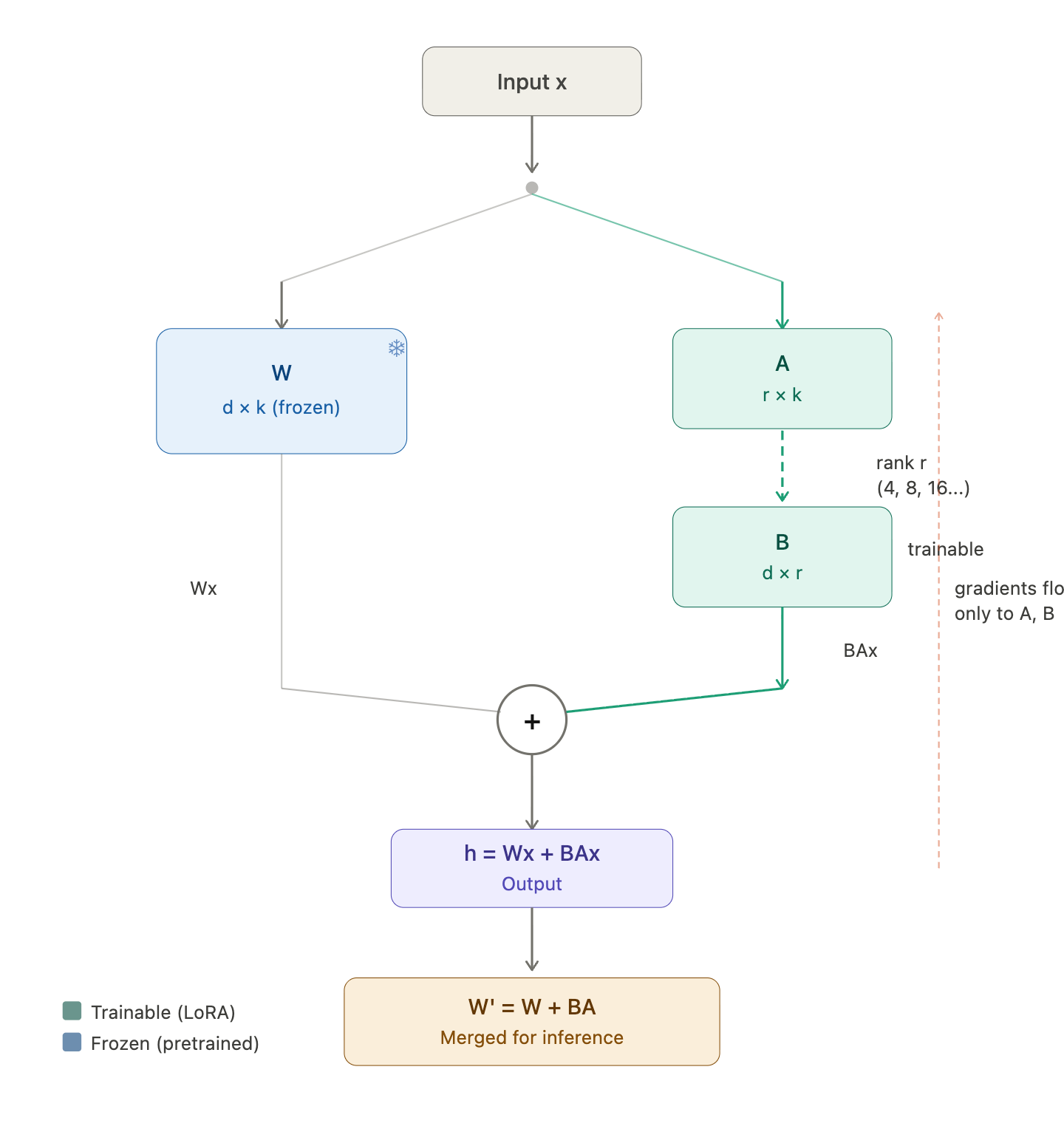 Fig. 2: LoRA training loop — the frozen weight W and the trainable adapters B × A run in parallel
-
Freeze the original weights. W is completely frozen — no gradients flow through it, and it never changes.
-
Forward pass. For an input x (the output from the previous layer), the output becomes: h = Wx + BAx. The original frozen path and the LoRA path run in parallel, and their outputs are summed — think of it as the original model’s output plus a small correction from the adapters.
-
Backward pass. Since W is frozen, gradients only flow back to A and B. The optimizer updates A and B by a tiny step in the direction that reduces the loss. W never changes.
-
Repeat the forward and backward passes until training is complete.
-
Merge. After training, we merge the LoRA weights back into the original: W’ = W + BA. Now we have a single weight matrix that combines the original pretrained knowledge with the fine-tuning adjustments.
#QLoRA
QLoRA stands for Quantized Low-Rank Adaptation — it combines the two techniques we have covered:
- Q = Quantized (the frozen weights are stored in 4-bit NF4)
- LoRA = Low-Rank Adaptation (the trainable A and B adapters)
The only difference from LoRA is one extra step during each forward pass:
LoRA: h = Wx + BAx
QLoRA: h = dequant(W_nf4)x + BAx
Before the frozen W gets multiplied with x, it has to be dequantized from 4-bit back to 16-bit on the fly. So QLoRA trades some computation speed for massive memory savings — the frozen base model takes up ~4x less VRAM, while the LoRA adapters still train in full precision.
#LoRA Hyperparameters
Now that we understand how LoRA works, here are the hyperparameters that control the adapters. We saw rank (r) and the matrices A and B earlier — these settings let us tune how much capacity and influence the adapters have.
| Hyperparameter | What it does | Typical value | Too high | Too low |
|---|---|---|---|---|
| LoRA rank (r) | Dimensionality of adapter matrices — how expressive the adapters are | 16 or 32 | More memory/compute, risk of overfitting | Not enough capacity to learn the task |
| LoRA alpha (α) | Scales how strongly adapters influence the output | 2 × r (so 32 or 64) | Adapters overpower base model | Adapters barely affect output |
| LoRA dropout | Dropout rate on adapter layers — regularization to prevent overfitting | 0.05–0.1 | Underfitting, adapters can’t learn enough | Overfitting on small datasets |
| Target modules | Which layers get LoRA adapters attached | q_proj, v_proj (attention layers) | More modules = more parameters, slower training | Fewer modules = less capacity to adapt |
Scaling factor. The LoRA output is actually scaled by α/r before being added, so the full forward pass is: h = Wx + (α/r) · BAx. Think of α/r as a volume knob for the adapters — it controls how much the adapter correction influences the final output. For example, with α = 32 and r = 16, the scaling factor is 2, meaning the adapter output is doubled before being added. This is why alpha is typically set to 2× the rank.
In practice, most of these hyperparameters have well-established defaults, so the LoRA configuration is straightforward for most fine-tuning tasks.
#Beyond LoRA
So when should we use LoRA over full fine-tuning?
Use LoRA when:
- We have limited GPU memory (most people)
- The task is narrow — classification, a specific output style, or domain adaptation
- We want fast iteration — LoRA trains faster and produces tiny adapter files
- We want to keep the base model intact and swap different adapters for different tasks
Consider full fine-tuning when:
- We have the compute resources (multiple high-end GPUs)
- The task requires deep changes to the model’s behavior across many capabilities
- Maximum performance matters more than efficiency
For most fine-tuning use cases, LoRA (or QLoRA) is the practical choice — it gets us most of the performance at a fraction of the cost.
That covers the concepts behind LoRA, quantization, and QLoRA. In the next article, I will walk through the actual training code — from loading the model to configuring LoRA and running the training loop.